Code Stream: The Program

We previously defined the code stream as consisting of “an ordered sequence of operations,” and this definition is fine as far as it goes. But in order to dig deeper, we need a more detailed picture of what the code stream is and how it works.

The term operations suggests a series of simple arithmetic operations like addition or subtraction, but the code stream consists of more than just arithmetic operations. Therefore, it would be better to say that the code stream consists of an ordered sequence of instructions.

Instructions are commands that tell the whole computer (not just the ALU, but multiple parts of the machine) exactly what actions to perform. As we’ve seen, a computer’s list of potential actions encompasses more than just simple arithmetic operations.

General Instruction Types

Instructions are grouped into ordered lists that, when taken as a whole, tell the different parts of the computer how to work together to perform a specific task, like grayscaling an image or playing a media file. These ordered lists of instructions are called programs, and they consist of a few basic types of instructions.

In modern RISC microprocessors, the act of moving data between memory and the registers is under the explicit control of the code stream, or program. So if a programmer wants to add two numbers that are located in main memory and then store the result back in main memory, he or she must write a list of instructions (a program) to tell the computer exactly what to do. The program must consist of:

a load instruction to move the two numbers from memory into the registers.
an add instruction to tell the ALU to add the two numbers.
a store instruction to tell the computer to place the result of the addition back into memory, overwriting whatever was previously there.

These operations fall into two main categories:

Arithmetic instructions

These instructions tell the ALU to perform an arithmetic calculation (for example, add, sub, mul, div).

Memory-access instructions

These instructions tell the parts of the processor that deal with main memory to move data from and to main memory (for example, load and store).

To show you how memory-access and arithmetic operations work together within the context of the code stream, we will use a series of increasingly detailed examples. All of the examples are based on a simple, hypothetical computer, which is called the DLW-1 (hypothetical processor is named by "Inside the Machine" book's author Jon Stocks)

The DLW-1’s Basic Architecture

The DLW-1 microprocessor consists of an ALU (along with a few other units) attached to four registers, named A, B, C, and D for convenience.

The DLW-1 is attached to a bank of main memory that’s laid out as a line of 256 memory cells, numbered #0 to #255 (The number that identifies an individual memory cell is called an address).

The DLW-1’s Arithmetic Instruction Format

All of the DLW-1’s arithmetic instructions are in the following instruction format:

instruction source1, source2, destination

There are four parts to this instruction format, each of which is called a field.

The field instruction specifies the type of operation being performed (for example, an addition, a subtraction, a multiplication, and so on).
The source fields source1 and source2 tell the computer which registers hold the two numbers being operated on (the operands).
the field destination tells the computer which register to place the result in.

As a quick illustration, an addition instruction that adds the numbers in registers A and B (the two source registers) and places the result in register C (the destination register) would look like this:

Code:
add A, B, C

Comment:
Add the contents of registers A and B and place the result in C, overwriting
whatever was previously there.

The DLW-1’s Memory Instruction Format

In order to get the processor to move two operands from main memory into the source registers so they can be added, you need to tell the processor explicitly that you want to move the data in two specific memory cells to two specific registers. This “filing” operation is done via a memory-access instruction called the load.

As its name suggests, the load instruction loads the appropriate data from main memory into the appropriate registers so that the data will be available for subsequent arithmetic instructions.

The store instruction is the reverse of the load instruction, and it takes data from a register and stores it in a location in main memory, overwriting whatever was there previously.

All of the memory-access instructions for the DLW-1 have the following instruction format:

instruction source, destination

For all memory accesses, the instruction field specifies the type of memory operation to be performed (either a load or a store).

In the case of a load, the source field tells the computer which memory address to fetch the data from, while the destination field specifies which register to put it in.
In the case of a store, the source field tells the computer which register to take the data from, and the destination field specifies which memory address to write the data to.

An Example DLW-1 Program

Now consider the below Program, which is a piece of DLW-1 code. Each of the lines in the program must be executed in sequence to achieve the desired result.

Program 1: Program to add two numbers from main memory
---------------------------------------------
load #12, A     Read the contents of memory cell #12 into register A.
load #13, B     Read the contents of memory cell #13 into register B.
add A, B, C     Add the numbers in registers A and B and store the result in C.
store C, #14    Write the result of the addition from register C into memory cell #14.

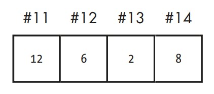
Suppose the main memory looked like the following before running Program 1:

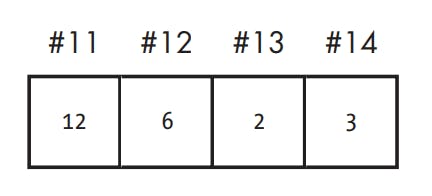
After doing our addition and storing the results, the memory would be changed so that the contents of cell #14 would be overwritten by the sum of cells #12 and #13.

Memory Accesses: Register vs. Immediate

The examples so far presume that the programmer knows the exact memory location of every number that he or she wants to load and store. In other words, it presumes that in composing each program, the programmer has at his or her disposal a list of the contents of memory cells #0 through #255.

While such an accurate snapshot of the initial state of main memory may be feasible for a small example computer with only 256 memory locations, such snapshots almost never exist in the real world. Real computers have billions of possible locations in which data can be stored, so programmers need a more flexible way to access memory, a way that doesn’t require each memory access to specify numerically an exact memory address.

Modern computers allow the contents of a register to be used as a memory address, a move that provides the programmer with the desired flexibility. But before discussing the effects of this move in more detail, let’s take one more look at the basic add instruction.

Immediate Values

All of the arithmetic instructions so far have required two source registers as input. However, it’s possible to replace one or both of the source registers with an explicit numerical value, called an immediate value.

For instance, to increase whatever number is in register A by 2, we don’t need to load the value 2 into a second source register, like B, from some cell in main memory that contains that value. Rather, we can just tell the computer to add 2 to A directly, as follows:

add A, 2, A     Add 2 to the contents of register A and place the result back into A,
                overwriting whatever was there.

We have actually been using immediate values all along in my examples, but just not in any arithmetic instructions. In all of the preceding examples, each load and store uses an immediate value in order to specify a memory address.

So, the #12 in the load instruction in line 1 of Program 1 is just an immediate value (a regular whole number) prefixed by a # sign to let the computer know that this particular immediate value is a memory address that designates a cell in memory.

Memory addresses are just regular whole numbers that are specially marked with the # sign. Because they’re regular whole numbers, they can be stored in registers and stored in memory just like any other number. Thus, the whole-number contents of a register, like D, could be construed by the computer as representing a memory address.

For example, say that we’ve stored the number 12 in register D, and that we intend to use the contents of D as the address of a memory cell in Program 2.

Program 2: Program to add two numbers from main memory using an address stored in
a register
--------------------------------------
load #D, A      Read the contents of the memory cell designated by the number
                stored in D (where D = 12) into register A.
load #13, B     Read the contents of memory cell #13 into register B.
add A, B, C     Add the numbers in registers A and B and store the result in C.
store C, #14    Write the result of the addition from register C into memory cell #14.

Program 2 is essentially the same as Program 1, and given the same input, it yields the same results. The only difference is in line 1:

Program 1, Line 1        Program 2, Line 1
load #12, A              load #D, A

Since the content of D is the number 12, we can tell the computer to look in D for the memory cell address by substituting the register name (this time marked with a # sign for use as an address), for the actual memory cell number in line 1’s load instruction. Thus, the first lines of Programs 1 and 2 are functionally equivalent.

This same trick works for store instructions, as well. For example, if we place the number 14 in D we can modify the store command in line 4 of Program 1 to read as follows: store C, #D. Again, this modification would not change the program’s output.

Because memory addresses are just regular numbers, they can be stored in memory cells as well as in registers. Program 3 illustrates the use of a memory address that’s stored in another memory cell. If we take the input for Program 1 and apply it to Program 1-3, we get the same output as if we’d just run Program 1 without modification:

Program 3: Program to add two numbers from memory using an address stored in a
memory cell.
------------------------------------
load #11, D     Read the contents of memory cell #11 into D.
load #D, A      Read the contents of the memory cell designated by the number in D
                (where D = 12) into register A.
load #13, B     Read the contents of memory cell #13 into register B.
add A, B, C     Add the numbers in registers A and B and store the result in C.
store C, #14    Write the result of the addition from register C into memory cell #14.

The first instruction in Program 1-3 loads the number 12 from memory cell #11 into register D. The second instruction then uses the content of D (which is the value 12) as a memory address in order to load register A into memory location #12.

But why go to the trouble of storing memory addresses in memory cells and then loading the addresses from main memory into the registers before they’re finally ready to be used to access memory again? Isn’t this an overly complicated way to do things?

Actually, these capabilities are designed to make programmers’ lives easier, because when used with the register-relative addressing technique, they make managing code and data traffic between the processor and massive amounts of main memory much less complex.

Register-Relative Addressing

In real-world programs, loads and stores most often use register-relative addressing, which is a way of specifying memory addresses relative to a register that contains a fixed base address.

For example, we’ve been using D to store memory addresses, so let’s say that on the DLW-1 we can assume that, unless it is explicitly told to do otherwise, the operating system always loads the starting address (or base address) of a program’s data segment into D.

Remember that code and data are logically separated in main memory, and that data flows into the processor from a data storage area, while code flows into the processor from a special code storage area. Main memory itself is just one long row of undifferentiated memory cells, each one byte in width, that store numbers. The computer carves up this long row of bytes into multiple segments, some of which store code and some of which store data.

A data segment is a block of contiguous memory cells that a program stores all of its data in, so if a programmer knows a data segment’s starting address (base address) in memory, he or she can access all of the other memory locations in that segment using this formula:

base address + offset

where offset is the distance in bytes of the desired memory location from the data segment’s base address.

Thus, load and store instructions in DLW-1 assembly would normally look something like this:

load #(D + 108), A     Read the contents of the memory cell at location #(D + 108) into A.
store B, #(D + 108)    Write the contents of B into the memory cell at location #(D + 108).

In the case of the load, the processor takes the number in D, which is the base address of the data segment, adds 108 to it, and uses the result as the load’s destination memory address.

Of course, this technique requires that a quick addition operation (called an address calculation) be part of the execution of the load instruction, so this is why the load-store units on modern processors contain very fast integer addition hardware.

By using register-relative addressing instead of absolute addressing (in which memory addresses are given as immediate values), a programmer can write programs without knowing the exact location of data in memory. All the programmer needs to know is which register the operating system will place the data segment’s base address in, and he or she can do all memory accesses relative to that base address. In situations where a programmer uses absolute addressing, when the operating system loads the program into memory, all of the program’s immediate address values have to be changed to reflect the data segment’s actual location in memory.

Because both memory addresses and regular integer numbers are stored in the same registers, these registers are called general-purpose registers (GPRs). On the DLW-1, A, B, C, and D are all GPRs.

Learner